Potts Model

In statistical mechanics, the Ising model is the standard introduction to phase transitions, describing spins that can be either “up” or “down” ($s_i\in \{-1,+1\}$). While powerful, it represents a specific universality class characterized by continuous, second-order phase transitions. To explore richer physics, such as discontinuous first-order transitions involving latent heat, we must generalize the model.

This leads us to the $q$-state Potts model.

Mathematical Foundations

In the Potts model, discrete variables living on lattice sites can take on one of $q$ distinct states (often visualized as “colors”): $s_i\in \{0,1,\dots ,q-1\}$. The interaction energy is defined such that energy is lowered only when neighboring spins are in the exact same state. The Hamiltonian is given by:

Here, $J>0$ is the ferromagnetic coupling constant, $⟨i,j⟩$ denotes nearest-neighbor pairs, and $\delta (s_i,s_j)$ is the Kronecker delta, which is 1 if $s_i=s_j$ and 0 otherwise.

A crucial feature of the 2D Potts model is that the nature of its phase transition changes depending on $q$. For $q\le 4$, the transition is continuous (second-order). For $q>4$, the transition becomes discontinuous (first-order). We selected $q=10$ for this simulation to clearly observe the sharp signatures of a first-order transition.

Simulation Methodology: The Swendsen-Wang Algorithm

Simulating systems near phase transitions using standard single-spin flip methods (like the Metropolis algorithm) is notoriously difficult due to “critical slowing down”—the correlation length diverges, and the time required to decorrelate the system grows rapidly.

To overcome this, we employed the Swendsen-Wang (SW) algorithm, a powerful Cluster Monte Carlo method. Instead of flipping individual spins, the SW algorithm identifies and flips entire “clusters” of interacting spins simultaneously. A single step involves:

1. Bond Formation: Iterating through the lattice and creating bonds between neighboring sites having the same spin value with probability $p=1-e^{-J/k_{B}T}$.
2. Cluster Identification: Using a Union-Find data structure to identify connected components formed by these bonds. These components are the “clusters.”
3. Cluster Flipping: Assigning a new, random state uniformly chosen from $\{0,\dots ,q-1\}$ to each cluster.

This approach drastically reduces autocorrelation times, allowing us to efficiently sample the equilibrium states even right at the critical temperature $T_c$.

Discussion of Results

The following dashboard presents a comprehensive analysis of the $q=10$ Potts model simulation near its critical temperature.

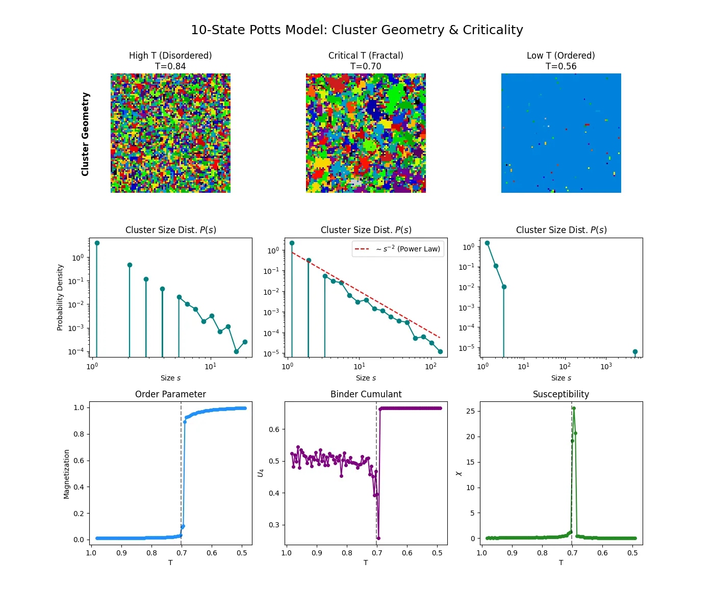
Row 1: Cluster Geometry Visualization

This row visualizes the actual clusters identified by the Swendsen-Wang algorithm at different temperatures. Colors represent distinct clusters.

• High T (Left): The system is disordered. Thermal noise prevents long-range bonds from forming, resulting in a fragmented landscape of tiny, disconnected clusters (“dust”).
• Critical T (Middle): At $T_c$, the system is poised at the percolation threshold. We observe fractal geometry and scale invariance—clusters of all sizes coexist, from single pixels to sprawling networks that nearly span the lattice.
• Low T (Right): The system has ordered. A single “giant component” (massive cluster) has percolated and dominates the entire system.

Row 2: Cluster Size Distribution $P(s)$

These log-log plots quantify the geometry seen in Row 1 by showing the probability distribution of cluster sizes, $s$.

• High T: The distribution shows a rapid downward curve, indicating exponential decay; large clusters are exponentially rare.
• Critical T: The data forms a nearly perfect straight line on the log-log plot. This indicates a power-law distribution ($P(s)\sim s^{-\tau }$), confirming the scale invariance and fractal nature of the clusters at the critical point.
• Low T: The distribution splits. A distinct “bump” appears at the far right of the plot ($s\approx {10}^3$ to ${10}^4$). This represents the macroscopic “infinite” cluster that has detached from the distribution of smaller fluctuations.

Row 3: Macroscopic Observables and First-Order Signatures

This row shows thermodynamic quantities as a function of temperature, revealing the discontinuous nature of the transition for $q=10$.

• Order Parameter (Magnetization): Unlike the smooth curve of the Ising model, the Potts order parameter shows a near-vertical “cliff” at $T_c$. The system jumps discontinuously from a disordered state ($M\approx 0$) to a highly ordered state.
• Binder Cumulant ($U_4$): This quantity is a definitive indicator of transition type. The sharp negative dip just before $T_c$ is the mathematical signature of a first-order transition, reflecting the coexistence of ordered and disordered phases and metastability.
• Susceptibility ($\chi$): We observe an extremely sharp, massive divergence at the critical temperature, indicating maximal fluctuations as the system undergoes the discontinuous jump.

Conclusion

By utilizing the efficient Swendsen-Wang cluster algorithm, we successfully simulated the $q=10$ Potts model and captured the defining characteristics of a first-order phase transition. The analysis provided a complete picture, linking the microscopic fractal geometry of percolating spin clusters to the resulting macroscopic discontinuities in the order parameter and the tell-tale negative dip in the Binder cumulant.