Trading simulation with the Ising Model.

by Lionel Yelibi, Feb 17, 2026

Standard economic theory often assumes markets are “efficient” and price changes follow a nice, bell-shaped Gaussian distribution. Anyone who has lived through 2008, 2020, or any major crypto cycle knows this is nonsense. Real markets are prone to massive bubbles, sudden crashes, and periods of intense volatility that standard models fail to predict.

This failure has given rise to Econophysics, a field that applies theories of statistical mechanics to financial markets. The core idea is simple but powerful: the collective behavior of traders panicking in a market looks suspiciously like the collective behavior of atoms aligning in a magnet.

In this post, we explore an Agent-Based Model (ABM) derived from the Ising Model of ferromagnetism to simulate trading behavior. We found that by combining simple behavioral rules with realistic network topologies, we can spontaneously reproduce the complex “stylized facts” of real financial markets.

The Physics of Fear and Greed

The Ising model explains how materials become magnetic. It describes a lattice of “spins” (atoms) that can point Up (+1) or Down (-1). Spins want to align with their neighbors to minimize energy, fighting against thermal noise ( $T$ ) that randomizes them.

The mapping to finance is remarkably direct:

Physics Concept	Financial Equivalent
Spin ( $s_{i} = \pm 1$ )	Trader Decision (+1 = Buy/Bull, -1 = Sell/Bear).
Coupling ( $J > 0$ )	Herding Behavior. The psychological pressure to copy peers (FOMO or panic).
Temperature ( $T$ )	Market Noise/Volatility. High $T$ means traders act randomly; Low $T$ means they lock into a consensus.
Magnetization ( $M$ )	Market Sentiment. The net imbalance of Buyers vs. Sellers, driving price changes.
Critical Point ( $T_{c}$ )	Phase Transition. The tipping point where a calm market suddenly herds into a crash or bubble.

Adding Dynamics: The Feedback Loop

A standard Ising model eventually settles into equilibrium. A real market never does. To create a dynamic trading simulator, we added a trend-following feedback loop.

We defined an “effective field” $H_{e f f}$ that acts on all traders, based on yesterday’s market movement:

H_{e f f} (t) = λ \cdot M (t - 1)

If the market went up yesterday ( $M > 0$ ), it creates a positive pressure to buy today. This simple rule, combined with neighbor imitation ( $J$ ), creates self-reinforcing trends—bubbles and crashes—that eventually collapse under their own weight or due to noise.

The Experiment: Topology Matters

In the real world, social influence isn’t a perfect grid. Some traders are isolated retail investors, while others are massive institutional hubs connected to everyone.

We simulated our Ising market on three different network topologies to see how connectivity shapes financial risk:

Lattice: A standard 2D grid (traders only see immediate physical neighbors).
Random Graph (Erdös-Rényi): Connections are completely random and uniform.
Scale-Free Network (Barabási-Albert): A realistic social network with “hubs” (influencers/banks) that are highly connected.

We swept temperatures to find the critical point for each network, and then ran deep simulations at the critical temperature to observe the dynamics.

Results: Reproducing Financial Reality

The results were striking. The topology of the trader network fundamentally dictated the “flavor” of the market dynamics.

The “Hero” Result: The Scale-Free Market

The scale-free network produced the most realistic financial data. Because “hubs” stabilize opinion, this network had a much higher critical temperature ( $T_{c} \approx 5.23$ ) than the others.

Dashboard showing the Scale-Free Ising Market simulation results.

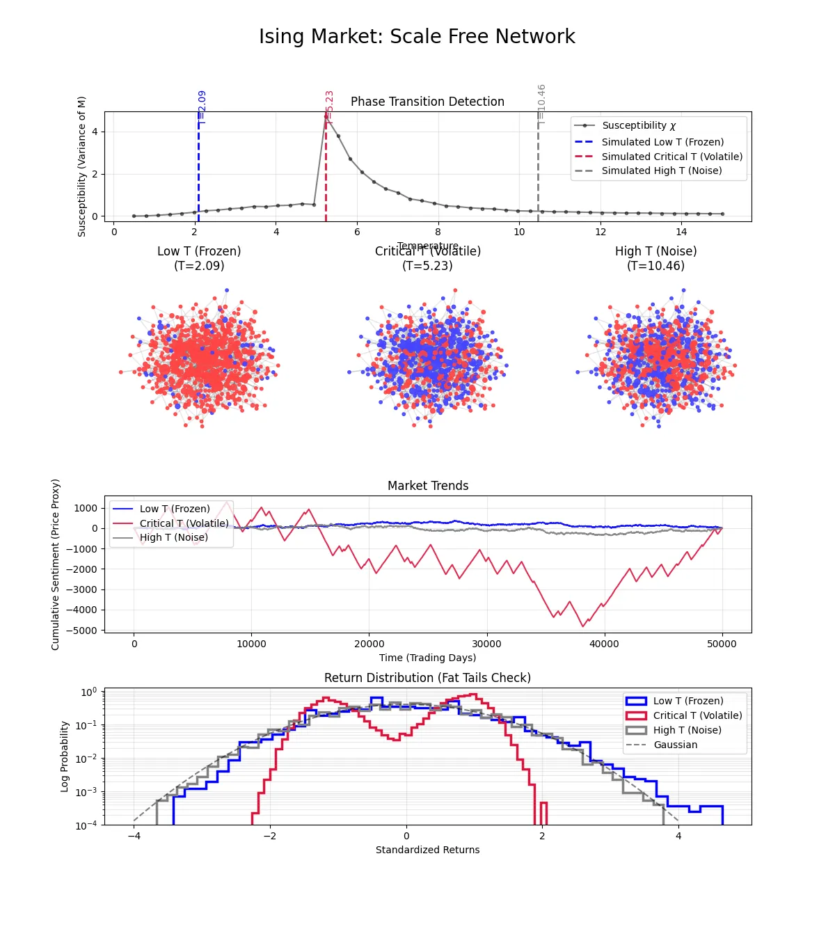
Fig 1: The Scale-Free Market dashboard. Row 1: Susceptibility peak identifying Tc. Row 2: Time series of sentiment. Row 3: Return distributions compared to a Gaussian.

Look at the Market Trends (Middle Row, Red Line). It doesn’t just oscillate randomly. It shows sustained trends—a massive “bear market” crash followed by a recovery. The jagged nature of the line shows volatility clustering: calm days are followed by calm days, and chaotic days by chaotic days.

Most importantly, look at the Return Distribution (Bottom Row). The gray dashed line is a standard Gaussian normal distribution. The red histogram is our simulation data.

It is unimodal (centered around zero change).
It has fat tails. The shoulders of the red histogram are much wider than the Gaussian. This means extreme events (3-sigma or 4-sigma moves) happen far more often than a random walk predicts.

This spontaneously reproduces the most important statistical characteristic of real asset returns.

Comparison: Lattice and Random Markets

In contrast, the other topologies produced less realistic markets at criticality.

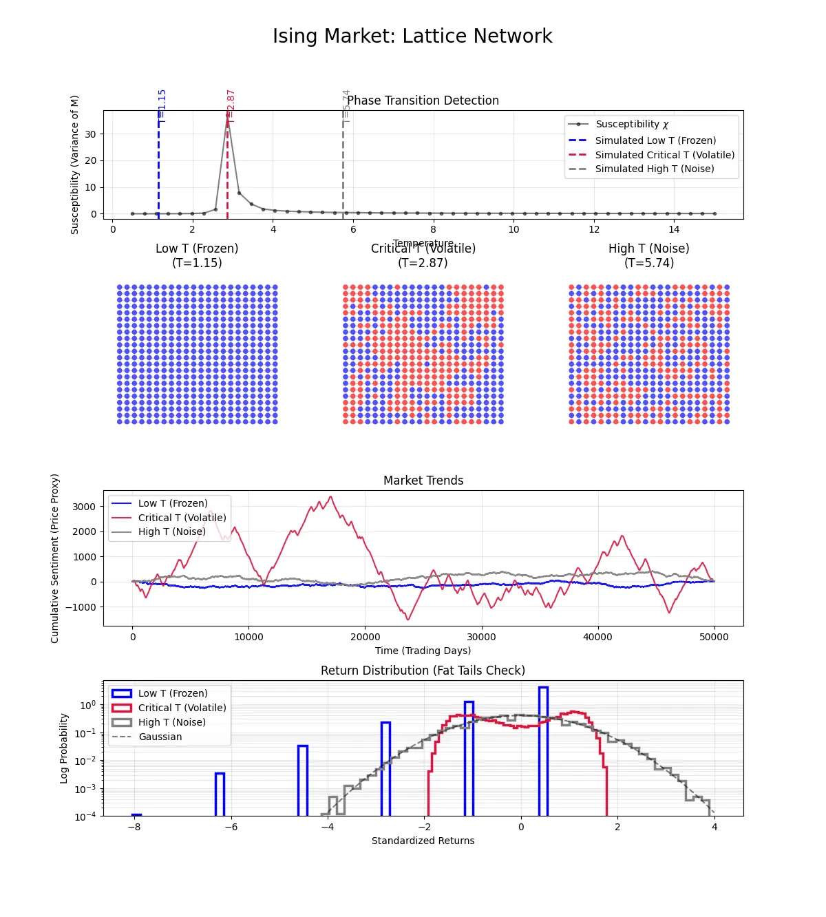
Dashboard showing the Lattice Ising Market results.

Fig 2: The Lattice Market. Note the bimodal (“two-humped”) distribution in the bottom row.

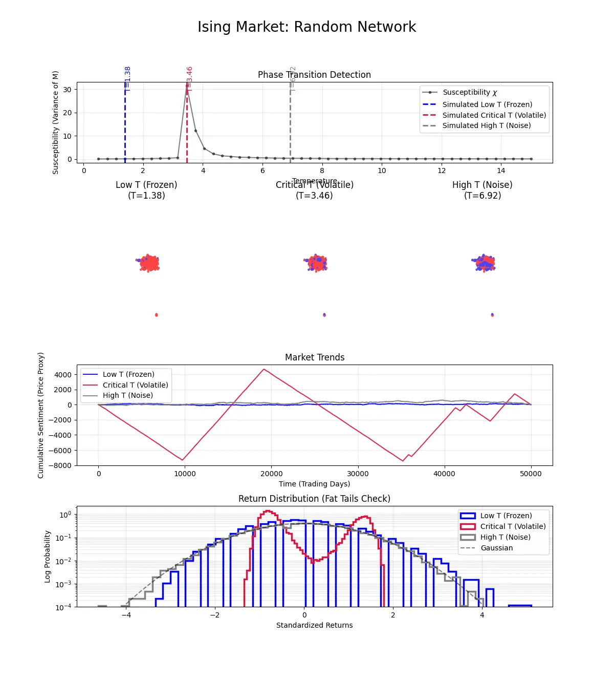
Dashboard showing the Random Graph Ising Market results.

Fig 3: The Random Graph Market. Also shows strong bimodal behavior.

In both the Lattice and Random graphs, the critical return distribution is bimodal. The market spends most of its time at extreme $+ 1$ (massive boom) or extreme $- 1$ (massive crash), rapidly switching between them.

While these show phase transitions, they don’t look like real stock markets, which spend most days near zero change. The Scale-Free network, with its realistic mix of hubs and isolated nodes, is required to get the nuanced, heavy-tailed behavior of real finance.

Conclusion

By stripping financial markets down to their physics bare essentials—imitation, noise, and trend following—we found that complex market dynamics emerge spontaneously. We didn’t program “crashes” into the model; they emerged as a natural consequence of agents interacting on a scale-free network near a critical point.

This demonstrates the power of econophysics: sometimes, to understand Wall Street, you need to think like a magnet.